NOTE:  The Dec 6 post is combined with this one from yesterday.  All targets remain unchanged from last week.

 *  *  *

Technical analysis encompasses a wide array of indicators — sentiment, flow, volume, open interest, moving averages, momentum, chart patterns and Fibonacci patterns.  Many fundamental analysts disparage the practice, but begrudgingly dabble when a signal is compelling enough.

Much has been written about the yield curve’s ability to forecast recessions — which sometimes helps one forecast markets. Many pundits seem to regard an inversion of the 2s10s as a sign of an impending correction — pointing to the current spread of 15bps with some alarm.

But, as we’ve discussed many times, it’s the rapid spike in the 2s10s following an inversion that is highly correlated with the biggest equity collapses of the past 20 years.It’s a good model, but not a perfect one.

In 2000, the yield curve low of -0.52 came on April 7, two weeks after SPX topped out.  By the time it reached 0.0 in January 2001, SPX had fallen 19%.  SPX bounced 8% over the next month or so.  But, as the 2s10s topped its 1999 highs, SPX’s troubles began anew.  It plunged 45% by October 2002, two months after 2s10s reached its 2002 high of 2.37.

Again, good but not perfect.  If spiking 2s10s produced corrections, why did stocks top out well before the 2s10s bottomed out and well before it spiked higher?  And, why did stocks bottom out in October even as the 2s10s continued higher until July 2003?

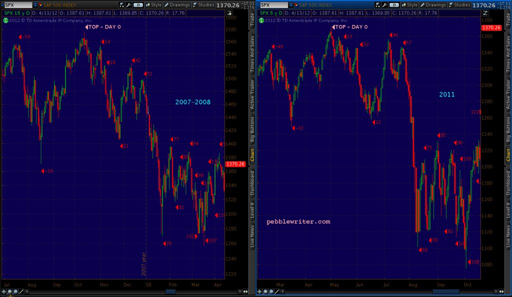
The 2007-2009 crash presented similar problems with the model. 2s10s inverted in January 2006, but bounced around between -0.19 and +0.21 until July 2007.  SPX didn’t top out until October 2007, at which point the 2s10s had already risen to 0.66.

SPX’s subsequent 58% collapse was nicely correlated with 2s10s.  But, again, the fit was far from perfect and there were numerous head fakes.

An examination of the 2Y and 10Y side by side in 2000-2002 shows that the sharp spike in 2s10s was primarily due to the relatively faster drop off in 2Y yields. 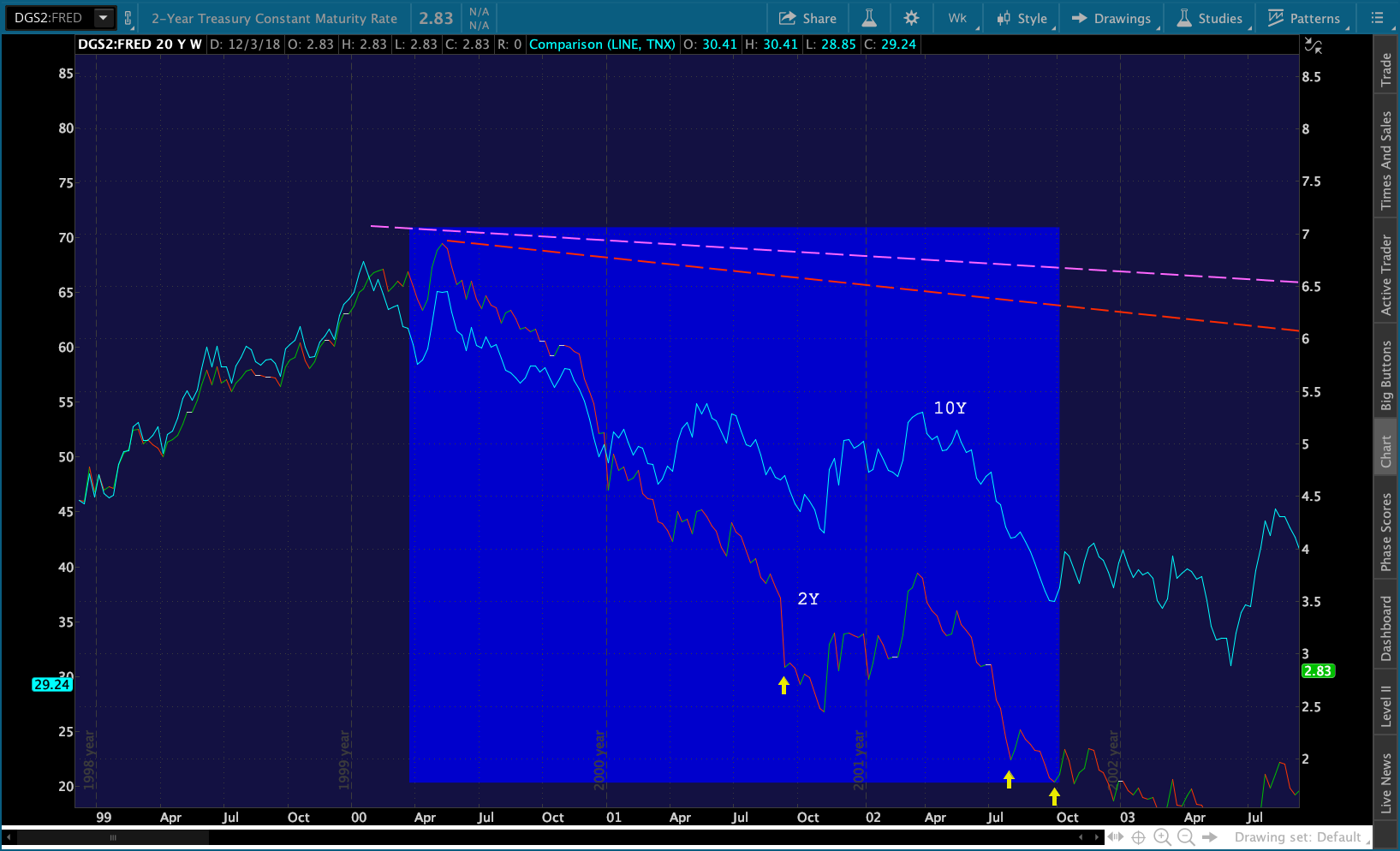 And, the sharpest drops in 2Y yields (the yellow arrows) matched up nicely with some of the sharpest drops in SPX.The same thing happened during the 2007-2009 crash.

The model thus becomes more robust: be wary of sharp rises in the 2s10s accompanied by sharp declines in the 2Y. But, it still doesn’t offer as much certainty as to timing as I’d like. And, as we discussed in our first post on the yield curve last year [see: Should You Fear the Yield Curve?] there have been other significant equity declines which were accompanied by sharp drops in the 2s10s.

Several additional posts over the past year have further developed the model, revealing several very interesting nuances that address both issues.  It has helped me pinpoint numerous interim turning points, including the recent 184-pt drop [see: Nov 9 Update.]

The basic rules can be observed on the chart below.  The colors refer to the arrows.(1) Bounces off trend lines (TLs) of support (purple, yellow) are generally bullish.
(2) Breakouts above TL of resistance (red) are bearish.
(3) Breakdowns below TLs (yellow and red) and horiz. support (white) are bearish.
(4) Reversals at TLs of resistance (green) are bullish.

Following these rules would have yielded the following long/short decisions between December 2017 and April 2018.

a. Dec 5, Dec 15 and Jan 3 – long
b. Jan 29, Feb 1 – short
c. Feb 9 – long
d. Mar 12, Mar 28 – short
e. Mar 29, Apr 17 – long
f. Apr 19 – short

Let’s overlay SPX and see how the model did.  The shaded areas are the periods during which the model signaled a long position.  The unshaded areas indicated shorts.

A buy and hold strategy between Dec 5 (a) and Apr 19 (f) would have yielded a 64-pt or 2.4% gain.  While going long and short per the model (based on closing prices) would have yielded a 1,110-pt or 42% gain.

There was one period when 2s10s bounced back above the white TL when signals were definitely mixed. But, since SPX was bouncing along atop its 200-DMA, it wasn’t tough to decipher the correct signal.

This was also clearly a period of extraordinarily large moves higher and lower.  So, the value of the signals was much greater than might otherwise have been the case.  Let’s take a look at the more recent case — between July 13 and the present.

A buy and hold strategy would have yielded a 101-pt or 3.6% loss.  The model, applying only the broad strokes, would have generated 740 points, or 26.4%.  And, since 2s10s just fell through horizontal support on Tuesday, there’s likely more downside ahead.

The yield curve model is only one component of our overall analysis.  And, the above both oversimplifies its application and understates its value.  Combined with the other tools I use every day, it’s contributing to a banner year.

 

continued for members…

Broad strokes from the most recent formation…  Note that 2s10s just dropped through the white support line, indicating further downside. The 2s10s won’t reach the red trend line until it reaches about 10 bps.  The purple TL is much lower, around 4 bps.  But, as we’ve seen from previous white TL breakdowns (the big red arrows below), the devil is in the details.  A clean breakdown as in Jun 2018 should produce a nice clean drop.  One that bounces back and forth across the support line as in March and April can produce a lot of chop. Picking up on a point made above, if the Fed follows through on the dovish comments Powell made last week, how long will it be until the 2Y starts to tumble?

I’ll continue this post tomorrow, Dec 6 when the markets reopen.

UPDATE:  Dec 6  8:00 AM

We’re seeing some nice follow through from Tuesday’s meltdown.  I have a follow up appointment with my oral surgeon this morning.  So, I’ll just post and dash.  Targets remain unchanged.

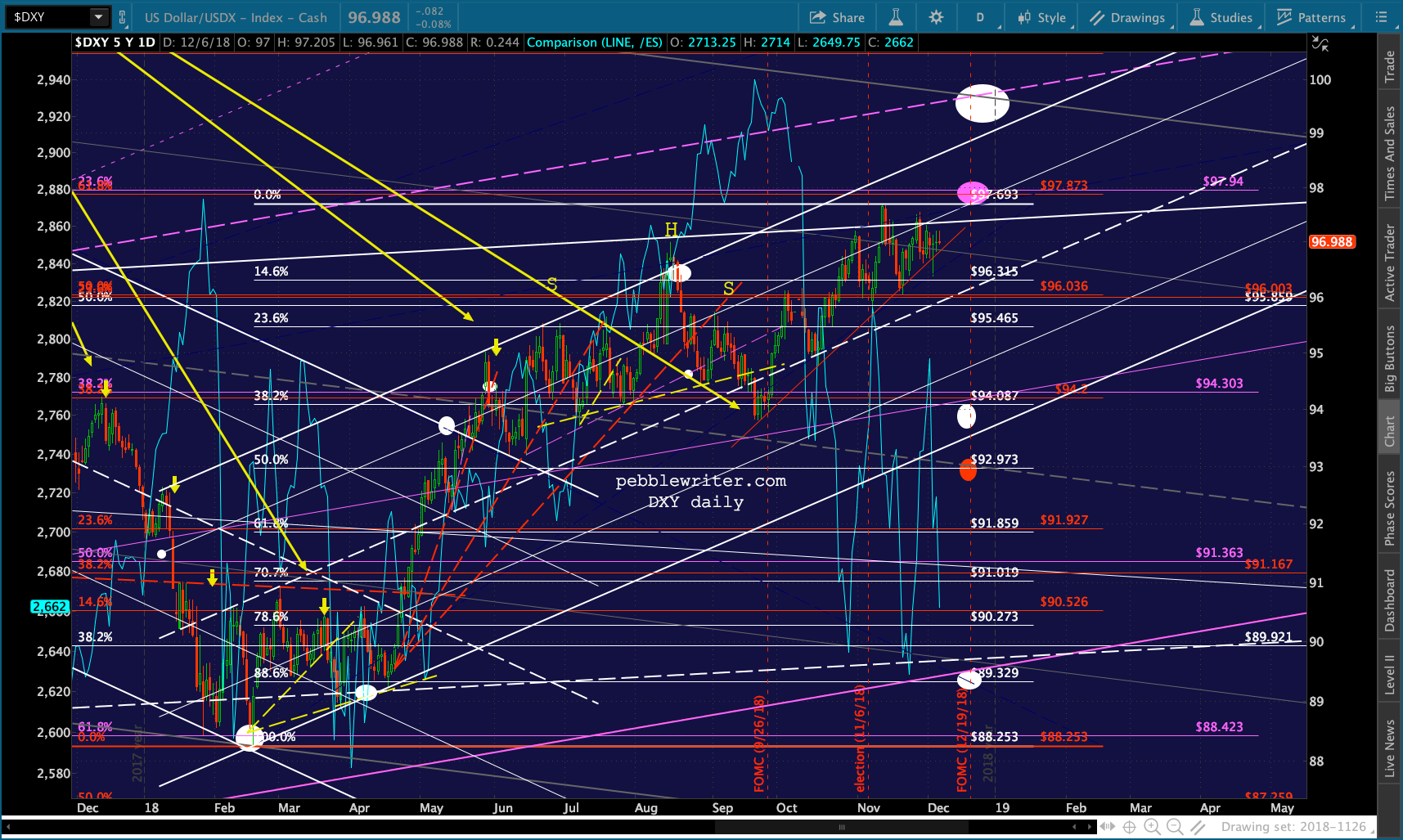
Futures are currently off about 40, but were as low as 2649 earlier.A reminder of the big picture:

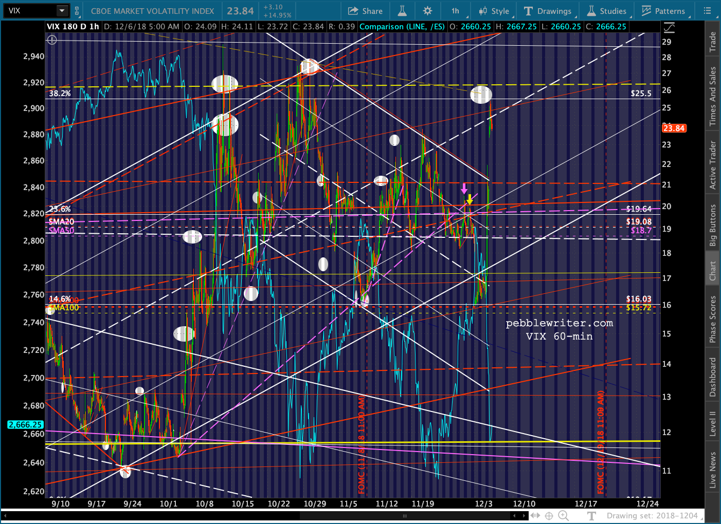Keep an eye on VIX.  If it breaks out past the 25.5 target, the next most likely target is the .618 at 34.97.As always, keep an eye on USDJPY as well.  A drop below the TL at 112 would be fuel to the fire.

RB and CL are showing weakness, but I continue to think CL is more vulnerable here. And, the bond market…  TNX has reached TL support, but has potential to push lower to the .382 and rising red TL. More later.

UPDATE:  2:10 PM

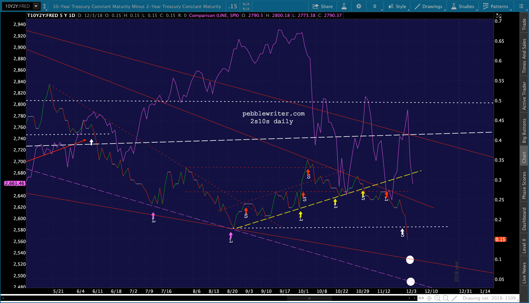
TNX just reached not only the .382, but very nearly the red TL.  I suspect it has a little further to go…… which means the 2s10s is probably due to invert any second. VIX reached the TL and reversed, which is putting a damper on additional SPX declines.

USDJPY is also getting a nice bounce off its TL.  SPX tagged its green .886 — an adequate drop — and bounced.  It missed the neckline and channel bottom by about 9 points.   At this point, it’s going to want to close the gap left at 2697.18.  And, the fact that it is about to experience a death cross must have some important feathers very ruffled. ES also came within about 10 points of thewhite channel bottom and neckline and is working on constructing a dragonfly candle.There is very little that TPTB can’t accomplish with manipulation of VIX and USDJPY — if they’re willing to part with the “cash” it takes to push them around.  CL and RB have even bounced off their earlier lows without having made new lows.  Rumor has it the Fed is going to be more dovish at their upcoming meeting.  We’ll see.  At this point, it seems that such an action would accelerate the yield curve’s inversion and put additional pressure on stocks.

Stay tuned.